Updated February 27, 2026
Pre-Calibration Product Known Issues
The NISAR project is still in the calibration and validation phase, and products released in the NISAR BETA collections were not yet fully calibrated. Through processing of the global data, the project learned about some unique characteristics of this first-of-a-kind radar system and has identified required algorithm updates. As a result, pre-calibration products have a number of features that are known to limit their use as science products and others that would be considered artifacts and are to be improved in future product releases.
Nonetheless, the BETA products are of sufficient quality to provide a useful look at the products from early acquisitions. Fully calibrated and algorithmically improved PROVISIONAL products are available as of July 2026.
Valid Data Mask
The mask that describes the fully-focused valid data region in all products is misaligned with the data. For example, as illustrated in Illustration of the valid data mask offset. for the Range/Doppler single look complex image, on the left side of the image, the subswath mask correctly captures the invalid region (black band) whereas on the right side, the invalid region is not correctly captured. This propagates to higher-level products.
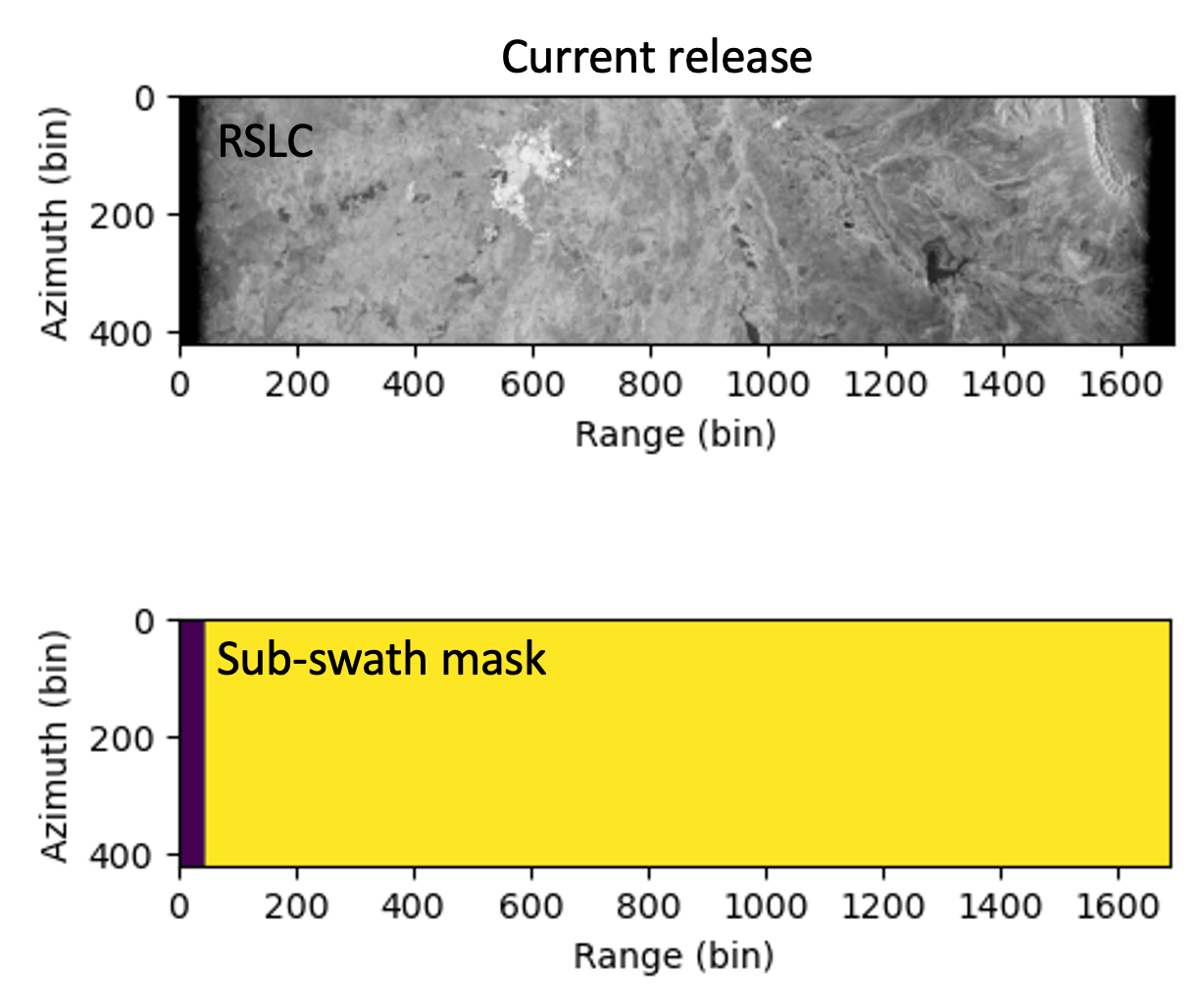
Illustration of the valid data mask offset.
Radiometric Banding
There is radiometric banding across the swath. This is due to incomplete calibration, specifically:
The effect of the cross-track antenna pattern for both co- and cross-polarized channels has not been completely removed. This will appear as bright and dark bands in the along-track dimension that can become most apparent in regions of uniform radar cross-section, such as tropical forests (Illustration of radiometric banding and misalignment of the data mask for co- and cross-polarized NISAR data. NISAR uses a “split spectrum” transmit waveform, creating two distinct radar bands for each observation.
Frequency Ais the main band, and typically has 20 MHz, 40 MHz or 77 MHz bandwidths centered at the lower end of the available spectrum.Frequency Bhas 5 MHz bandwidth at the upper end of the spectrum.Frequency Bdata is used for this illustration, as the banding is more prominent than inFrequency Adata.).
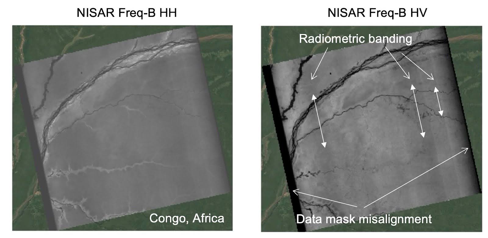
Illustration of radiometric banding and misalignment of the data mask for co- and cross-polarized NISAR data. NISAR uses a “split spectrum” transmit waveform, creating two distinct radar bands for each observation. Frequency A is the main band, and typically has 20 MHz, 40 MHz or 77 MHz bandwidths centered at the lower end of the available spectrum. Frequency B has 5 MHz bandwidth at the upper end of the spectrum. Frequency B data is used for this illustration, as the banding is more prominent than in Frequency A data.
There may be parallel streaks in the cross-track direction (Parallel streaks in cross-track direction in very low backscatter areas (here shown in RSLC HV Frequency A).) and/or in the along-track direction (Parallel streaks in along-track direction in very low backscatter areas (here shown in GCOV HH Frequency B).) visible in very low backscatter areas (i.e. lakes, sandy desert areas, etc.) in enhanced visualizations, especially visible in HV polarization.
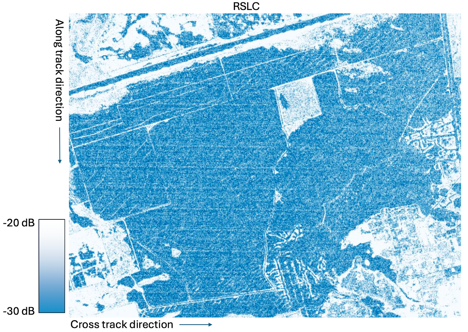
Parallel streaks in cross-track direction in very low backscatter areas (here shown in RSLC HV Frequency A).
Parallel streaks in along-track direction in very low backscatter areas (here shown in GCOV HH Frequency B).
Radio Frequency Interference (RFI)
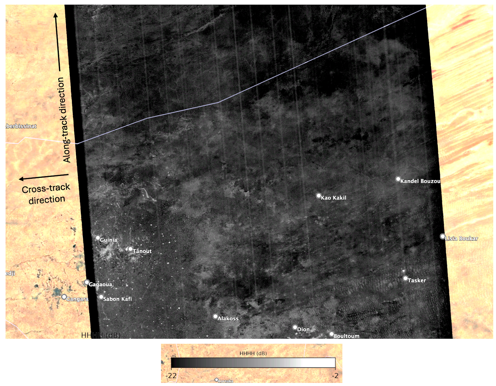
Backscatter data and interferograms can be affected by RFI. RFI signatures typically appear as bright blobs in polarimetric backscatter imagery and high decorrelation in the coherence and interferograms, or sharp bands oriented along the range direction, as seen in Examples of Radio Frequency Interference (RFI) over different regions. These types of interference become more evident in regions of low radar reflectivity, especially for cross-polarized (e.g. HV) returns..
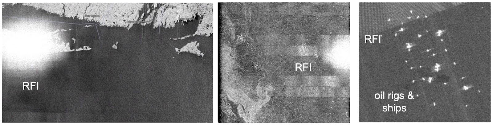
Examples of Radio Frequency Interference (RFI) over different regions. These types of interference become more evident in regions of low radar reflectivity, especially for cross-polarized (e.g. HV) returns.
Changes in Radar Acquisition Modes
Changes in the radar acquisition mode within a frame will lead to multiple partial frame image products for the same frame.
Noise Floor
The noise floor for 77 MHz data appears higher than expected. This issue is still being investigated, but is probably related to the calibration tone settings and how they impact quantization.
Interferometric Products
Ionospheric Correction Layer
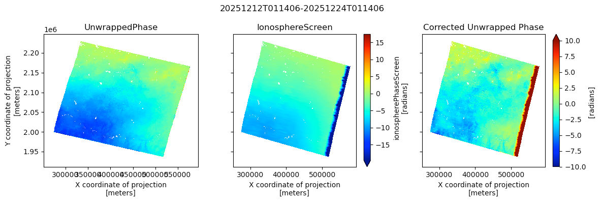
Some interferograms and range/Doppler offset products can exhibit very strong ionospheric signatures, such as decorrelation streaks and high-rate fringes because we are near the solar maximum of the solar cycle. A separate ionospheric estimate layer is provided for correction.
This layer compensates ionospheric phase quite well in low to mid-latitudes where ionospheric effects are moderate, but residual ionospheric signatures may remain, particularly in descending tracks (evening) and at all times in higher latitudes, where ionospheric effects can be more pronounced.
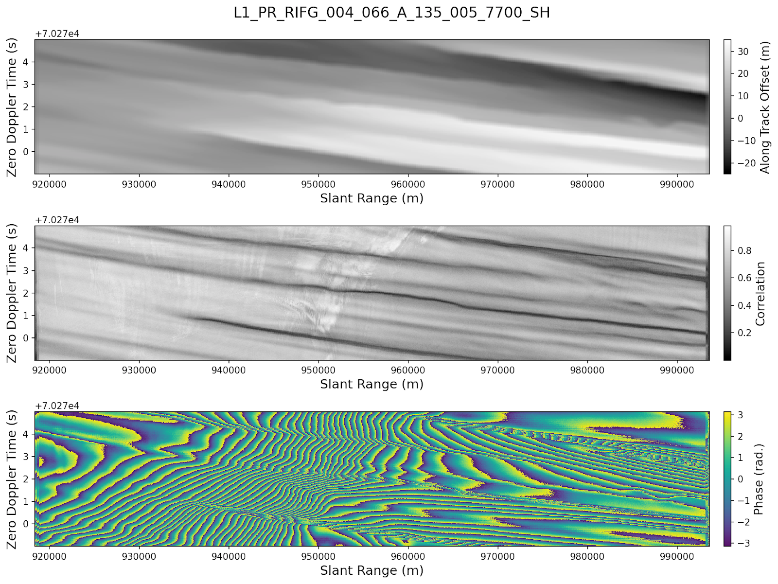
Along-track pixel offset estimates (top), the interferometric correlation (middle) and the interferometric phase (bottom) near Crary Ice Rise in Antarctica.
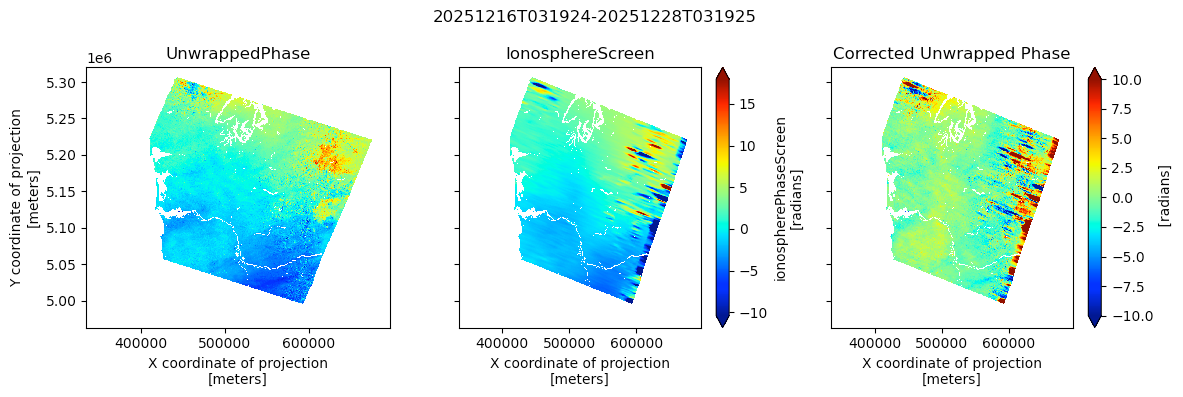
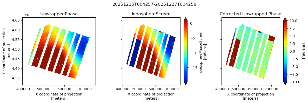
The boundary of the ionospheric phase layer has edge-effect artifacts, as illustrated in Edge-effect artifacts at the boundary of the ionospheric phase layer.. These artifacts originate from misaligned valid sample subswath masks in the input RSLC products.
Edge-effect artifacts at the boundary of the ionospheric phase layer.
Ionospheric phase layers may show localized artifacts due to Radio Frequency Interference (RFI), and decorrelation due to water bodies, vegetation, snow coverage or other factors. The algorithm refinement to mitigate or better mask such localized decorrelating regions and minimize artifacts in the ionospheric phase is under development.
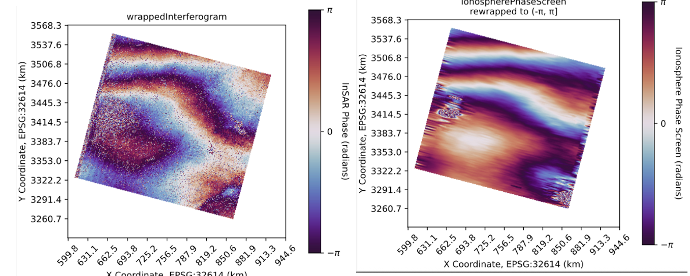
Illustration of localized artifacts in the ionospheric phase screen, which can be caused by RFI or decorrelation.
Ionosphere Phase Estimation can be affected by the masking of the transmit gaps in Frequency A and Frequency B. If gaps and noise around these gaps are not masked well in one of two frequencies, it will cause unwrapping errors and distort the ionospheric phase screens.
Phase unwrapping errors caused by the transmit gaps.
Valid Data Mask
The subswath mask indicating the valid region of the fully focused imagery is not fully aligned. This mask layer is provided to mask out unreliable data. Artifacts on the edges of many L2 geocoded products (GSLC, GUNW and GCOV) are therefore exposed, as illustrated in Misalignment of the subswath valid data mask causes edge effects in many of the L2 geocoded products..
Misalignment of the subswath valid data mask causes edge effects in many of the L2 geocoded products.
Rubbersheeting Algorithm
Interferograms with very strong deformation signals or ionospheric activity may contain artifacts because interferograms over solid earth regions do not yet use the full “rubbersheeting” algorithm to estimate local image distortions due to large, local, image pixel movements (Illustration of artifacts caused by not using the full rubbersheeting algorithm to estimate local image distortions due to large, local, image pixel movements.).
The algorithm used here for alignment of radar imagery (coregistration) is based on geometrical offsets (derived from imaging geometry of the NISAR acquisitions, orbit, and a digital elevation model) refined with a polynomial fit to the data-driven dense offsets computed from amplitude cross correlation of the radar data.
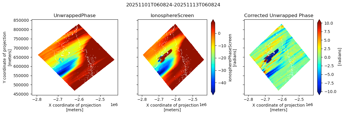
Illustration of artifacts caused by not using the full rubbersheeting algorithm to estimate local image distortions due to large, local, image pixel movements.
Interferogram Coregistration in Cryosphere Regions
Interferogram generation over cryosphere regions uses a rubbersheeting algorithm in which the coregistration is based on geometrical offsets refined with dense offsets computed from amplitude cross correlation. The ionosphere can introduce errors of a few pixels in the azimuth direction, which can yield an additional phase distortion beyond the direct effect of ionosphere on the phase.
Banding in Interferograms
Individual ionospheric phase screens contain banded phase artifacts oriented along the range direction due to mismatched ionosphere filtering. This banding is magnified in interferogram stacks, as illustrated in Stack of ionosphere-corrected interferograms displaying banded phase artifacts. Color scale is in radians.. While this problem will be fixed in future releases, users can mitigate this effect in the pre-calibration data with further low-pass filtering of the provided ionospheric layer.
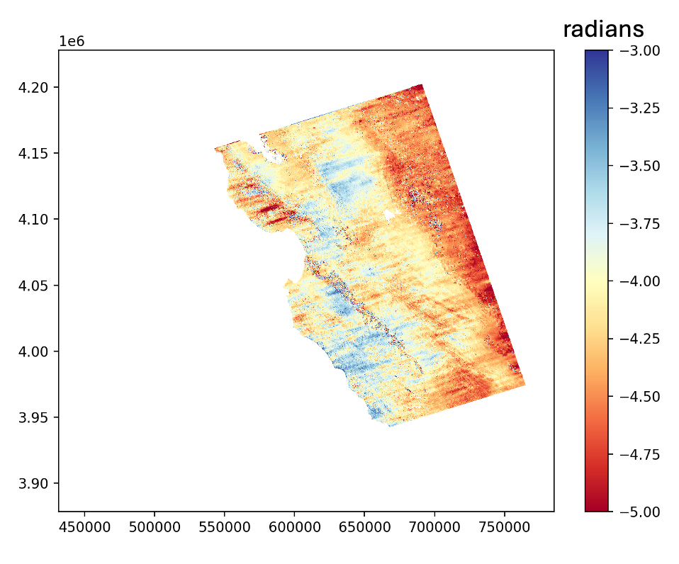
Stack of ionosphere-corrected interferograms displaying banded phase artifacts. Color scale is in radians.
ROFF Products
Range Doppler Pixel Offsets (ROFF) products for the ice sheets have severe, uncorrected ionospheric distortions in the azimuth offsets of up to a few pixels. In addition, the search radius used for offset tracking was too small to capture some fast motion (greater than a few thousand meters per year). The search radius will be expanded to capture the full range of motion in past and future acquisitions.
Soil Moisture (SME2)
The soil moisture retrievals are using uncalibrated lower level products, and therefore are not representative of the expected quality. Calibration continues on both the lower level products and the SME2 product itself. With large parts of the northern hemisphere frozen in the range of dates included in this release, calibration activities will continue well into the year.
It is recommended that investigators focus on the baseline soil moisture product (the
/science/LSAR/SME2/grids/soilMoisturevariable in the SME2 HDF5 files)Surface and retrieval flags included in the products have not been fully implemented, resulting in null values in the baseline layer.
Quad-Pol Product Noise Layers
In the Quad-Polarimetric (QP) products, the noiseEquivalentBackscatter layer for the HH polarimetric channel is currently populated with zeros. The noiseEquivalentBackscatter layers for the HV and VV polarimetric channels are populated with correct (uncalibrated) values.
Browse Image Geolocation
While each of the granules are well-geolocated (to within 5 m), the quick-look browse products can be mislocated up to many kilometers due to projection limitations in the kml browse products. As of this time, the 5 m geolocation errors may become apparent in some of the high resolution (40 MHz and above) and radiometrically terrain corrected GCOV images. A small geolocation offset in the descending image (top) from the DEM results in an error in the radiometric terrain correction. Meanwhile, in the ascending image (bottom), the radiometric terrain correction is correctly aligned with the DEM and the topographic variability is no longer evident. shows pixel misregistration.
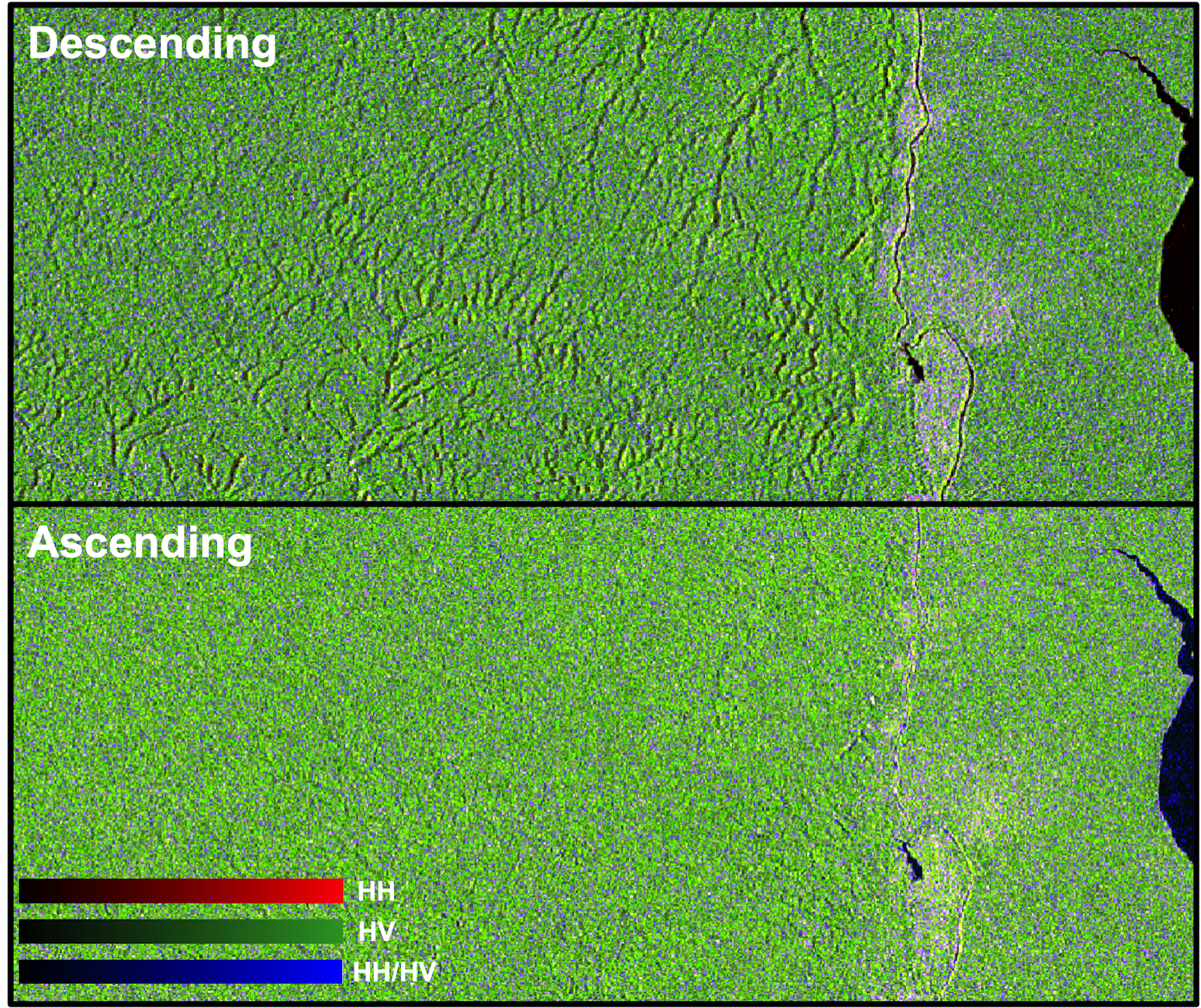
A small geolocation offset in the descending image (top) from the DEM results in an error in the radiometric terrain correction. Meanwhile, in the ascending image (bottom), the radiometric terrain correction is correctly aligned with the DEM and the topographic variability is no longer evident.