NISAR Level 2 and Level 3 products are projected to map coordinates and are suitable for use in QGIS. There is no minimum version required to work with NISAR data in QGIS, but this document was created using a QGIS version of 3.44.7.
For a refresher on available Level 2 and Level 3 NISAR data products, see Data Products Overview. To explore workflows for working with each specific NISAR data type in QGIS, see the Work with NISAR Sample Data tutorials.
A video tutorial demonstrating working with NISAR products in QGIS is available in the NISAR Science Team Town Hall and Data Access Webinar starting at timestamp 1:11:57.
Preparing NISAR Data for QGIS
QGIS cannot natively read the geolocation data of NISAR HDF5 files. A NISAR .h5 file loaded directly into QGIS will not display in the correct place on Earth.
Replacing the .h5 (HDF5) file extension with .nc (NETCDF) prior to opening the file in QGIS will allow the data to be correctly geolocated. For example, the file NISAR_L2_PR_GCOV_010_164_A_035_4005_DHDH_A_20260120T134235_20260120T134312_X05010_N_F_J_001.h5 renamed as NISAR_L2_PR_GCOV_010_164_A_035_4005_DHDH_A_20260120T134235_20260120T134312_X05010_N_F_J_001.nc can be opened in QGIS.
Occasionally, data files with an .nc extension may crash QGIS, but this can usually be fixed by deleting the .aux.xml file created by QGIS in the same directory as the dataset.
Preparing GSLC Products
QGIS cannot display complex-valued data such as the signal returns in NISAR GSLC products. The amplitude and phase components can be extracted into separate real-valued rasters using gdal_translate in conjunction with the derived subdatasets driver, which can then be visualized in QGIS. Amplitude data is typically more relevant than phase data for GIS applications.
Run the following example to extract the amplitude from a GSLC file:
gdal_translate -of GTiff DERIVED_SUBDATASET:AMPLITUDE:NETCDF:/path/to/nisar.nc:/science/LSAR/GSLC/grids/frequencyA/HH amplitude.tif
Now, amplitude.tif will be the file that can be loaded in QGIS.
Adding NISAR Data
Add data to QGIS using the Open Data Source Manger button and selecting the Raster data type. Select your NISAR file using the file explorer and click Add as shown in Figure 1.
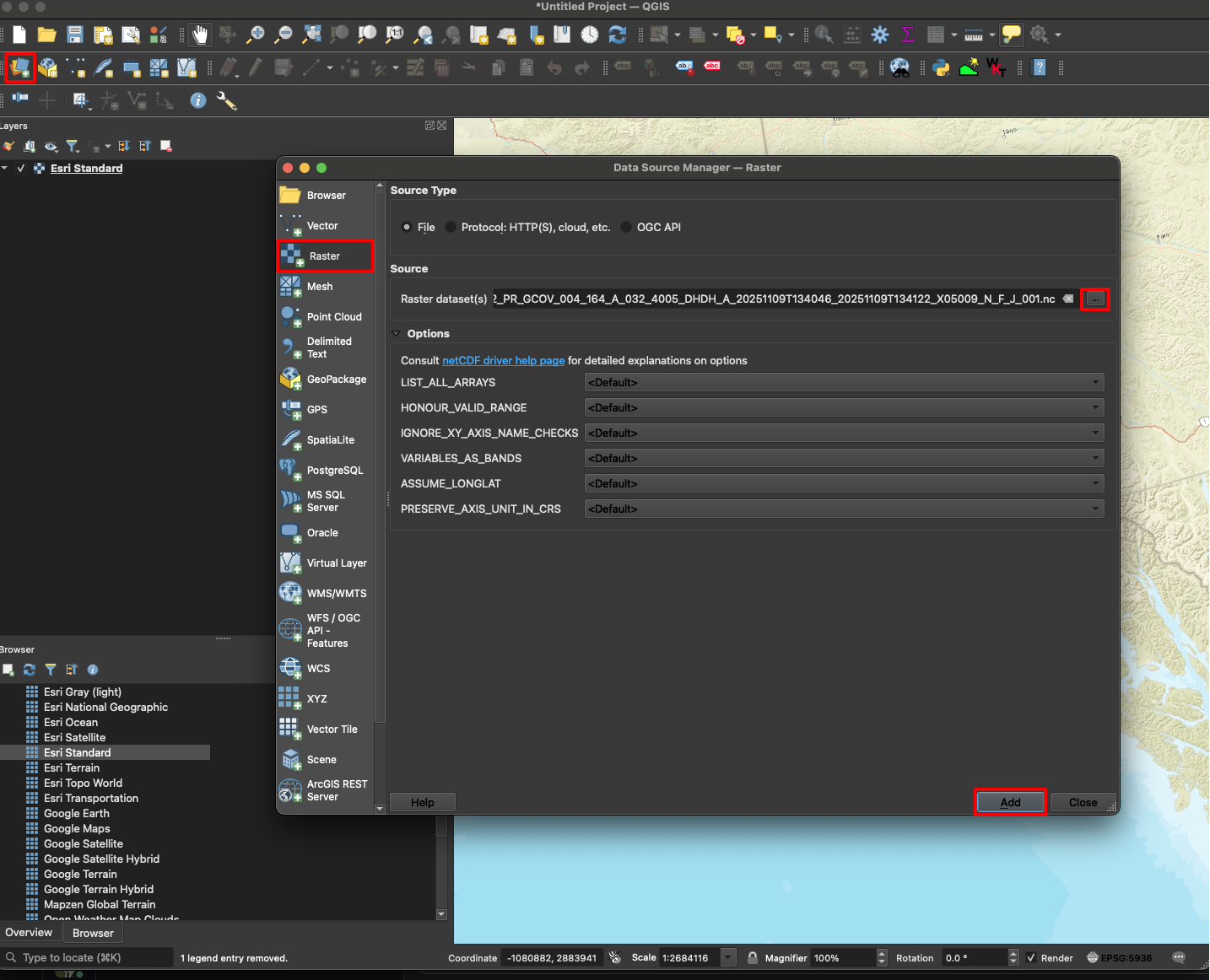
Figure 1:Click on Open Data Source Manger and select the Raster data type to add NISAR data to QGIS.
After clicking the Add button, another window will pop up showing a list of datasets within the NISAR data file that can be added as individual layers. All datasets are selected for addition by default, but you may want to select just a few of the available datasets to avoid adding too much data to your project.
For more information about the HDF file structure, see What is HDF5?.
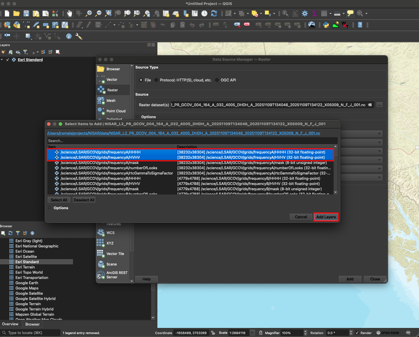
Figure 2:Select the data layers to add in QGIS. All layers are selected by default; highlight specific layers to add only the datasets you want.
Visualizing NISAR Data
After loading data into QGIS, the symbology needs to be adjusted to visualize the data in a meaningful way.
Right-click on a layer in the Layers Panel and select Properties to open the Layer Properties window. Click on the Symbology tab to access stretch and color ramp settings.
Stretch Settings
The stretch settings need to be adjusted to a smaller range of values in order to highlight the features in the scene. The minimum and maximum stretch values can be set by expanding Min/Max Value Settings in the Layer Properties window, as shown in Figure 3.
The minimum and maximum values can be User-defined to apply custom values, set by Cumulative count cut, which cuts a percentage of the highest and lowest values, set to the Min / Max values of the raster, or set to use the Mean +/- standard deviation.
There is no optimal universal approach for defining the minimum and maximum values; consider trying out different stretch settings to determine what works best for a specific image or application.
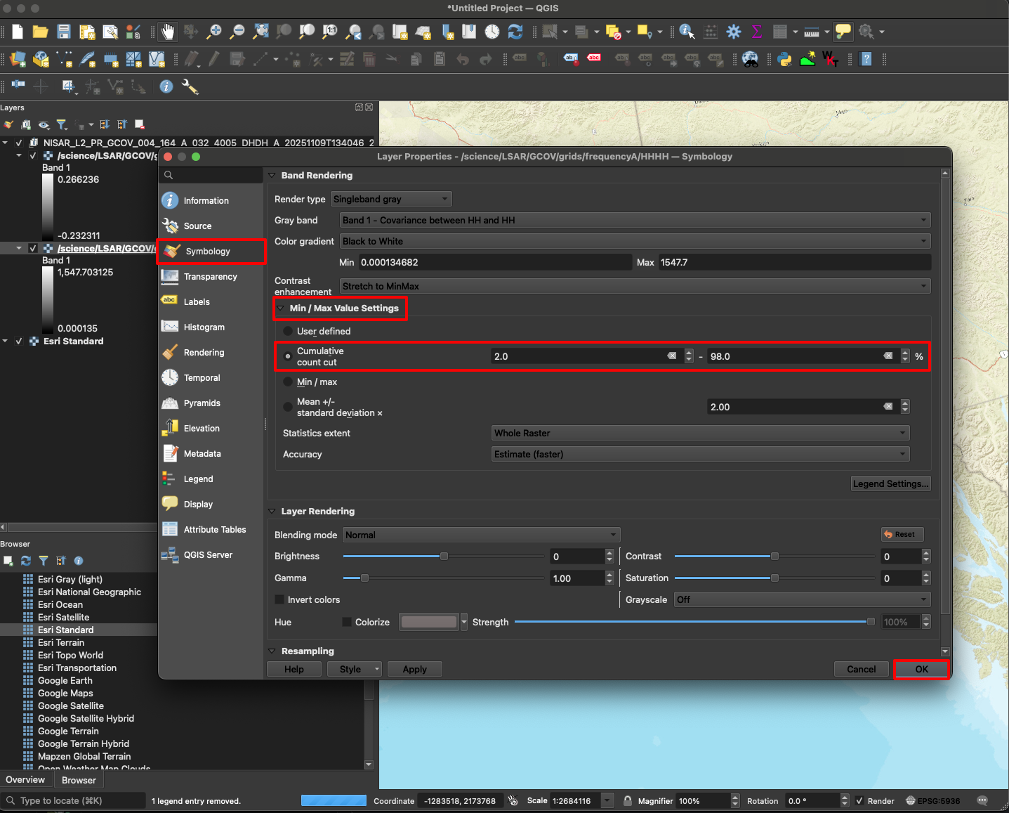
Figure 3:Right-click on the data layer in the Layers panel and select Properties to open up the Layer Properties window. Select the Symbology tab to customize stretch values for the gradient. Click OK to apply the symbology and close the Layer Properties window. In this example, a cumulative count cut stretch is applied.
Note that co-polarized (HHHH or VVVV) backscatter returns are generally higher than cross-polarized (HVHV or VHVH) returns. If you are setting the Min/Max values manually, the maximum value might need to be different depending on the polarization of the layer. The minimum value can be set to 0 for all polarizations.
Color Ramp Settings
NISAR data products will be displayed using a black and white (Singleband gray) color ramp in QGIS by default, but the color ramp can be changed in the Layer Properties window.
A variety of color ramps are available by changing the Render Type to Singleband pseudocolor, such as the Rocket color ramp, as seen in Figure 4.
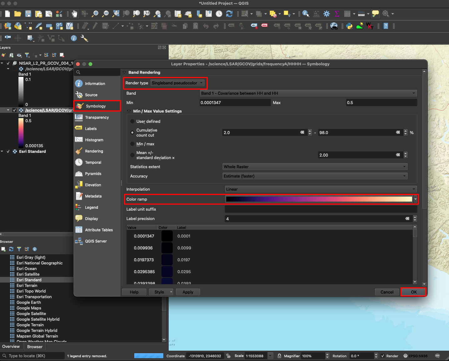
Figure 4:Right-click on the data layer in the Layers panel and select Properties to open up the Layer Properties window. Select the Symbology tab and change the Render Type to Singleband pseudocolor to change the Color ramp of the scene. In this example, the color ramp is set to Rocket.
Transforming NISAR Data
Subsetting
Raster data can be subset spatially in QGIS using the Clip Raster by Extent tool, as highlighted in Figure 5. Navigate to Raster on the menu bar, then select Extraction from the drop-down list to access this tool.
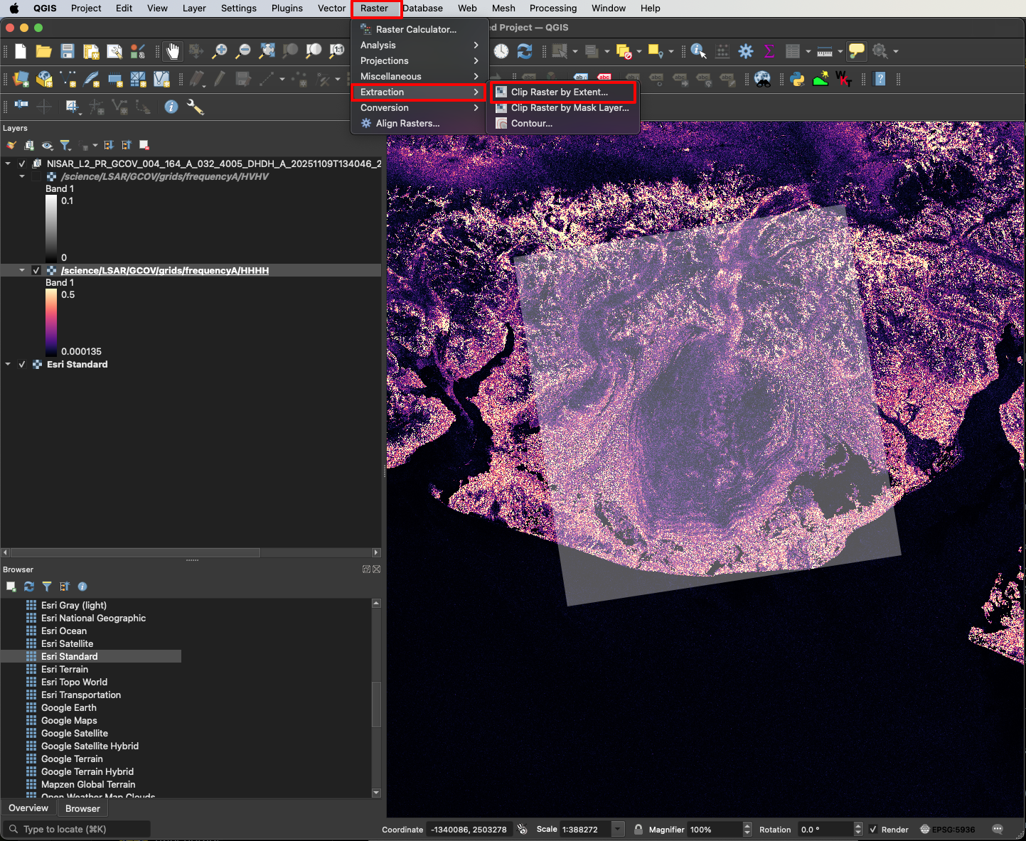
Figure 5:Select Raster from the menu bar, then select Extraction to open the Clip Raster by Extent raster tool.
Ensure the correct layer is selected under Input layer before subsetting. Set the extent of the desired subset using one of the available options. You can zoom to the extent of the desired subset and use the Use Current Map Canvas Extent option, select Draw on Map Canvas to draw a custom rectangle directly on the map, use the extent of another layer/bookmark/layout in your project, or type in the min/max XY coordinates and projection manually.
If you want to save the output raster to a file for use in other projects, set the path for the output file under the Clipped (extent) field in place of [Save to temporary file]. Click Run in the Raster Extraction window to generate the subset.
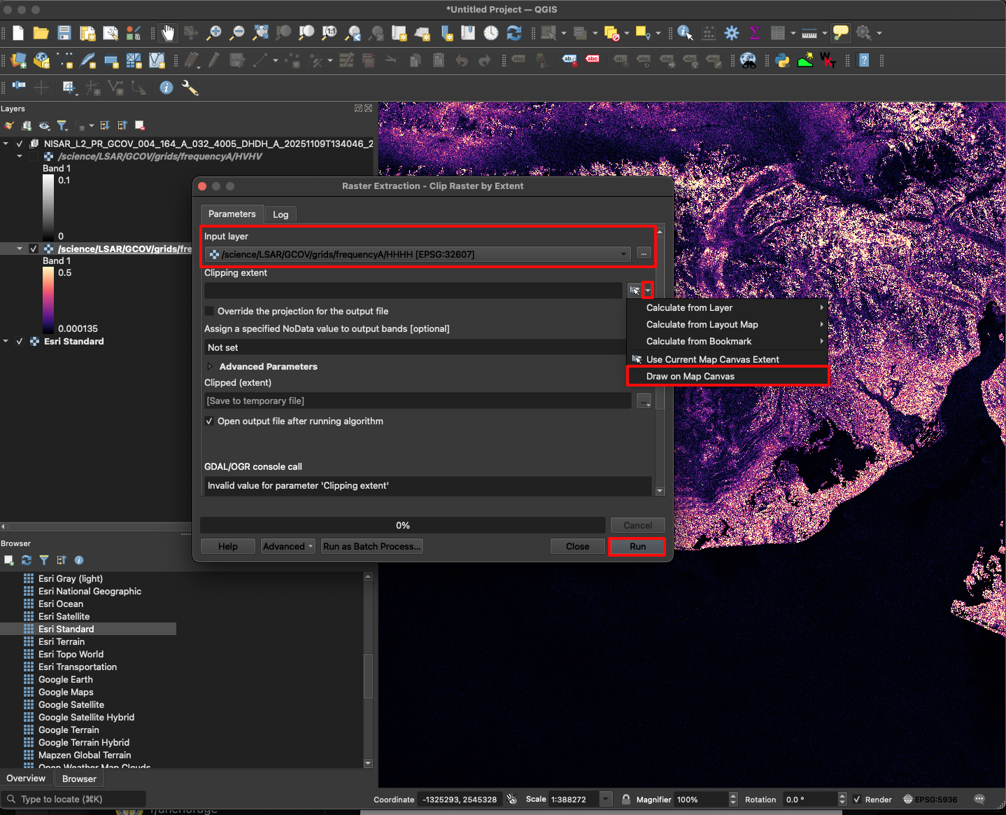
Figure 6:The Clip Raster by Extent tool has the option to draw a rectangle directly on the map, as illustrated here, along with many other options for setting the desired extent. Users can either save directly to a file or produce a temporary layer, which can later be saved.
Converting Format
Once a layer is ready to be exported, right-click on the layer in the Layers panel and select Export from the pop-up menu. Then, select Save As... from the pop-up list.
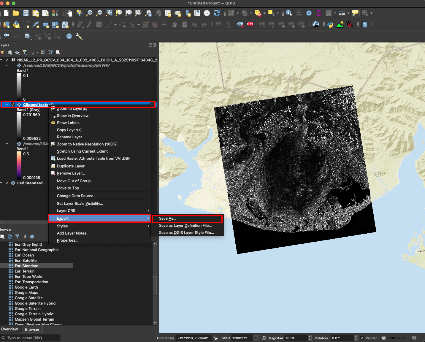
Figure 7:Right-click on a layer, select the Export option, then select Save As... to save it to another file format.
Select the desired output file type using the Format drop-down menu. Saving the layer as a GeoTIFF should be appropriate for most users. If desired, a different projection can be selected for the output file using the CRS menu. Input the desired name and location for the output file and press OK to save.
Note that you can also set a spatial extent during the export process rather than running a separate subsetting tool first.
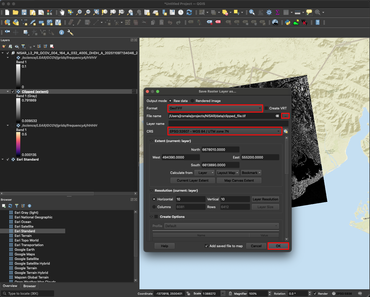
Figure 8:Select the output data format and a location and name for the file. Optionally, set a different projection and spatial extent for the output raster. Click OK to export the raster.